16 KiB
16 KiB
Data analytics: Feature engineering
- Data analytics: Feature engineering
Definition
- The process that attempts to create additional relevant features from existing raw features, to increase the predictive power of algorithms
- Alternative definition: transfer raw data into features that better represent the underlying problem, such that the accuracy of predictive model is improved.
- Important to machine learning
Sources of features
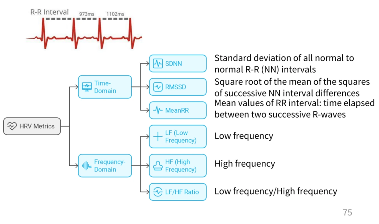
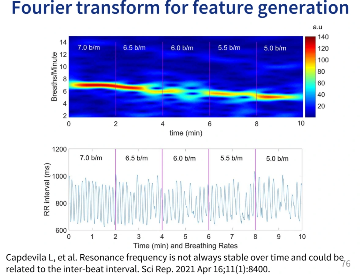
- Different features are needed for different problems, even in the same domain
Feature engineering in ML
- Process of ML iterations:
- Baseline model -> Feature engineering -> Model 2 -> Feature engineering -> Final
- Example: data needed to predict house price
- ML can do that with sufficient feature
- Reason for feature engineering: Raw data are rarely useful
- Must be mapped into a feature vector
- Good feature engineering takes the most time out of ML
Types of feature engineering
- Indicator variable to isolate information
- Highlighting interactions between features
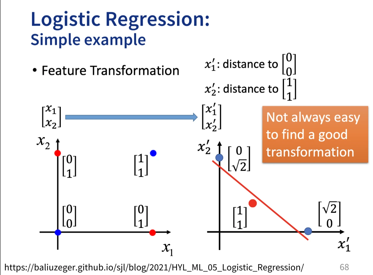
- Representing the feature in a different way
Good feature:
Related to objective (important)
- Example: the number of concrete blocks around it is not related to house prices
Known at prediction-time
- Some data could be known immediately, and some other data is not known in real time: Can't feed the feature to a model, if it isn't present at prediction time
- Feature definition shouldn't change over time
- Example: If the sales data at prediction time is only available within 3 days, with a 3 day lag, then current sale data can't be used for training (that has to predict with a 3-day old data)
Numeric with meaningful magnitude:
- It does not mean that categorical features can't be used in training: simply, they will need to be transformed through a process called encoding
- Example: Font category: (Arial, Times New Roman)
Have enough samples
- Have at least five examples of any value before using it in your model
- If features tend to be poorly assorted and are unbalanced, then the trained model will be biased
Bring human insight to problem
- Must have a reason for this feature to be useful, needs subject matter and curious mind
- This is an iterative process, need to use feedback from production usage
Methods of Feature Engineering
Scaling
Rationale:
- Leads to a better model, useful when data is uneven:
X1 >> X2
Methods:
Normalization or Standardization:
𝑍 = \frac{𝑋−𝜇}{\sigma}- Re-scaled to have a standard normal distribution that centered around 0 with SD of 1
- Will compress the value in the narrow range, if the variable is skewed, or
has outliers.
- This may impair the prediction
Min-max scaling:
X_{scaled} = \frac{X - min}{max - min}- Also will compress observation
Robust scaling:
X_{scaled} = \frac{X - median}{IQR}- IQR: Interquartile range
- Better at preserving the spread
Choosing
- If data is not guassain like, and has a skewed distribution or outliers : Use robust scaling, as the other two will compress the data to a narrow range, which is not ideal
- For PCA or LDA(distance or covariance calculation), better to use Normalization or Standardization, since it will remove the effect of numerical scale, on variance and covariance
- Min-Max scaling: is bound to 0-1, has same drawback as normalization, and new data may be out of bound (out of original range). This is preferred when the network prefer a 0-1 scale
Discretization / Binning / Bucketing
Definition
- The process of transforming continuous variable into discrete ones, by creating a set of continuous interval, that spans over the range of variable's values
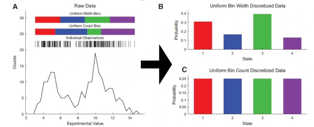
Reason for binning
- Example: Solar energy modeling
- Acceleration calculation, by binning, and reduce the number of simulation needed
- Improves performance by grouping data with similar attributes and has similar predictive strength
- Improve non-linearity, by being able to capture non-linear patterns , thus improving fitting power of model
- Interpretability is enhanced by grouping
- Reduce the impact of outliers
- Prevent overfitting
- Allow feature interaction, with continuous variables
Methods
Equal width binning
- Divide the scope into bins of the same width
- Con: is sensitive to skewed distribution
Equal frequency binning
- Divides the scope of possible values of variable into N bins, where each bin carries the same number of observations
- Con: May disrupt the relationship with target
k means binning
- Use k-means to partition the values into clusters
- Con: need hyper-parameter tuning
decision trees
- Using decision trees to decide the best splitting points
- Observes which bin is more similar than other bins
- Con:
- may cause overfitting
- have a chance of failing: bad performance
Encoding
Definition
- The inverse of binning: creating numerical values from categorical variables
Reason
- Machine learning algorithms require numerical input data, and this converts categorical data to numerical data
Methods
One hot encoding
- Replace categorical variable (nominal) with different binary variables
- Eliminates ordinality: since categorical variables shouldn't be ranked, otherwise the algorithm may think there's ordering between the variables
- Improve performance by allowing model to capture the complex relationship within the data, that may be missed if categorical variables are treated as single entities
- Cons
- High dimensionality: make the model more complex, and slower to train
- Is sparse data
- May lead to overfitting, especially if there's too many categories and sample size is small
- Usage:
- Good for algorithms that look at all features at the same time: neural network, clustering, SVM
- Used for linear regression, but keep k-1 binary variable to avoid
multicollinearity:
- In linear regression, the presence of all k binary variables for a categorical feature (where k is the number of categories) introduces perfect multicollinearity. This happens because the k-th variable is a linear combination of the others (e.g., if "Red" and "Blue" are 0, "Green" must be 1).
- Don't use for tree algorithms
Ordinal encoding
- Ordinal variable: comprises a finite set of discrete values with a ranked ordering
- Ordinal encoding replaces the label by ordered number
- Does not add value to give the variable more predictive power
- Usage:
- For categorical data with ordinal meaning
Count / frequency encoding
- Replace occurrences of label with the count of occurrences
- Cons:
- Will have loss of unique categories: (if the two categories have same frequency, they will be treated as the same)
- Doesn't handle unseen categories
- Overfitting, if low frequency in general
Mean / target encoding
- Replace the value for every categories with the avg of values for every category-value pair
- monotonic relationship between variable and target
- Don't expand the feature space
- Con: prone to overfitting
- Usage:
- High cardinality (the number of elements in a mathematical set) data, by leveraging the target variable's statistics to retain predictive power
Transformation
Reasons
- Linear/Logistic regression models has assumption between the predictors and
the outcome.
- Transformation may help create this relationship to avoid poor performance.
- Assumptions:
- Linear dependency between the predictors and the outcome.
- Multivariate normality (every variable X should follow a Gaussian distribution)
- No or little multicollinearity
- homogeneity of variance
- Example:
- Some other ML algorithms do not make any assumption, but still may benefit from a better distributed data
Methods
- Logarithmic transformation:
log(𝑥 + 1)- Useful when applied to skewed distributions, it expands small values and compress big values, helps to make the distribution less skewed
- Numerical values x must be
x \gt -1
- Reciprocal transformation
1/𝑥 - Square root
\sqrt{x}- Similar to log transform
- Exponential
- Box cox transformation
(x^\lambda - 1) / \lambda- prerequisite: numeric values must be positive, can be solved by shifting
- Quantile transformation: using quartiles
- Transform feature to use a uniform or normal distribution. Tends to spread out the most frequent values.
- This is robust
- But is non-linear transform, may distort linear correlation, but variables at different scales are more comparable
Generation
Definition
- Generating new features that are often not the result of feature transformation
- Examples:
Methods
Feature Crossing
- Create new features from existing ones, thus increasing predictive power
- Takes the Cartesian product of existing features
A\times B=\{(a,b), a \in A \ and\ b\in B\}.
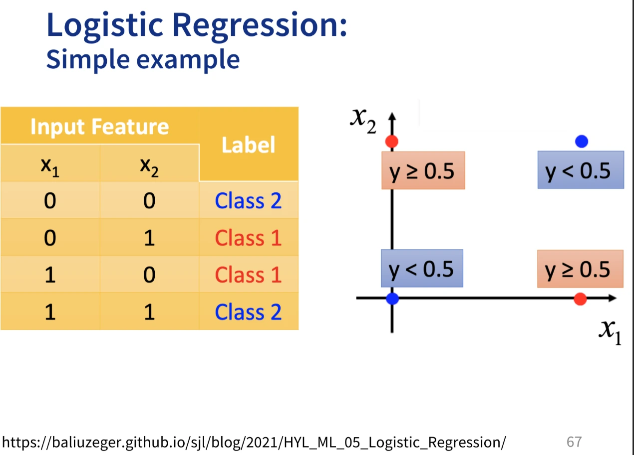
- Has uses when data is not linerarly separable
- Deciding which feature to cross:
- Use expertise
- Automatic exploration tools
- Deep learning
Polynomial Expansion
- Useful in modelling, since it can model non-linear relationships between predictor and outcome
- Use fitted polynomial variables to represent the data:
𝑝𝑜𝑙𝑦(𝑥, 𝑛)= 𝑎_0 + 𝑎_1 \times 𝑥 + 𝑎_2 \times 𝑥^2 + ⋯ + 𝑎_𝑛 \times 𝑥^𝑛
- Pros:
- Fast
- Good performance, compared to binning
- Doesn't create correlated features
- Good at handling continuous change
- Cons:
- Less interpretable
- Lots of variables produced
- Hard to model changes in distribution
Feature Learning by Trees
- Each sample is a leaf node
- Decision path to each node is a new non-linear feature
- We can create N new binary features (with N leaf nodes)
- Pro: Fast to get informative feature
Automatic Feature learning: Deep learning
- Deep learning model learns the features from data
- Difference between shallow networks
- Deep, in the sense of having multiple hidden layers
- Introduced stochastic gradient descent
- Can automate feature extraction
- Require larger datasets
- DL can learn hierarchical of features: Character → word → word group → clause → sentence
- CNN: use convolutional layers to apply filters to the input image, to detect various features such as edges, textures and shapes
Feature Selection
Reason
- More features doesn't necessarily lead to better model
- Feature selection is useful for
- Model simplification: easy interpretation, smaller model, less cost
- Lower data requirements: less data is required
- Less dimensionality
- Enhanced generalization, less overfitting
Methods
Filter
- Select best features via the following methods and evaluate
- Main methods
- Variance: remove the feature that has the same value
- Correlation: remove features that are highly correlated with each other
- Con: Fail to consider the interaction between features and may reduce the predict power of the model
Wrapper
- Use searching to search through all the possible feature subsets and evaluate them
- Steps of execution (p98), skipped
- Con: Computationally expensive
Embedded
- Use feature selection as a part of ML algorithm
- This address the drawbacks of both filter and wrapper method, and has advantage of both
- Faster than filter
- More accurate than filter
- Methods:
- Regularization: Add penalty to coefficients, which can turn them to zero, and can be removed from dataset
- Tree based methods: outputs feature importance, which can be used to select features.
Shuffling
Hybrid
Dimensionality Reduction
- When dimensionality is too high, it's computationally expensive to process them. We project the data to a lower subspace, that captures the essence of data
- Reason
- Curse of dimensionality: high dimensionality data have large number of features or dimensions, which can make it difficult to analyze and understand
- Remove sparse or noisy data, reduce overfitting
- To create a model with lower number of variables
- PCA:
- form of feature extraction, combines and transforms the dataset's original values
- projects data onto a new space, defined by this subset of principal components
- Is a unsupervised linear dimensionality reduction technique
- Preserves signal, filter out noise
- Use covariance matrix
- TODO: is calculation needed
- Minimize intraclass difference
- LDA:
- Similar to PCA
- Different than PCA, because it retains classification labels in dataset
- Goal: maximize data variance and maximise class difference in the data.
- Use scatter matrix
- Maximizes interclass difference
